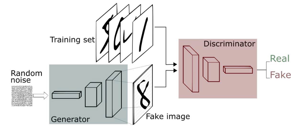
Generative Adversarial Networks, the Counterfeiter and the Police Game

Let’s picture the next game; two individuals, an outstanding counterfeiter who is well known for producing the best fake bills ever made, and the other hand, police, who are responsible for identifying whether the money moving around is real or fake. Such a play, isn’t it? We can cast Tom and Leo for the movie, right?
How is this related to Machine Learning, Deep Learning, or any Automated Learning known by humankind?
Deep learning promises to discover rich, hierarchical models that represent probability distributions over the kinds of data encountered in artificial intelligence applications, such as natural images, audio waveforms containing speech, and symbols, among others. We dreamed about Deep Learning implementations that can create content by themselves, and that my friends, is part of this journey. We are just starting, but the outcomes of different papers and researchers and promising. However; let’s start with something relatively simple that will help us to understand how Deep Learning solutions that can “Create” content. That’s why we will introduce our main character, Generative Adversarial Networks (GANs).
A Generative Adversarial Network (GAN) is a type of neural network architecture for carrying out generative modeling tasks proposed by Goodfellow et al in 2014. (Yeap, I need to come up with an article on Neural Networks, TBD)
Generative modeling involves the use of a model that aims to create
new examples are likely to come from an existing distribution of samples
but in turn, will be different from an existing population of instances, so those are fake (Synthetic).
A GAN is trained from two network architecture models. A generator (our counterfeiter) that learns to create new samples and a discriminator(our police) that learns to identify real/fake instances.
The goal of a GAN is that new content generated from noise in the
input is realistic enough to confuse the discriminator.
After training, the generative model will be able to create new synthetic samples and the discriminator should be able to identify real and fake inputs on demand. Sounds cool, right?
How GANs works?
As we mentioned, the generator tries to generate content realistic enough to deceive the discriminator. The goal of the discriminator is to discern the real content created by the generator from random noise.
In the end, it is a min-max game in which they compete among themselves, i.e. an adversarial task.
Now, you may be wondering, are images created from noise? From the architecture point of view, we refer to these as random values which serve as input to a low-dimensionality dense layer in charge of transforming the data into something more complex when transferring such information to a convolutional layer.
These architectures are designed based on state of art guidelines and algorithms. You will see many different implementations of generators and discriminators, and all of them work for specific tasks. Our goal here is just to give you a sense of how this technology works and provide you with tools to build your first GAN at home with a few lines. Don’t worry, we will walk you through every step.
GAN Training
The training of a GAN is carried out in two main phases.
The discriminator receives images from the generator and the real sample data and should learn to correctly discern both types of images. When the discriminator incorrectly tags an image, its weights are updated accordingly and the generator is notified about whether the image is good enough.
With the weights of the discriminator frozen, the generator introduces fake images with the label 1-Real to the discriminator. When the discriminator predicts that the image is false because the label does not match the prediction, the discriminator triggers a notification to update the weights of the generator which leads to the synthesis of increasingly realistic images.
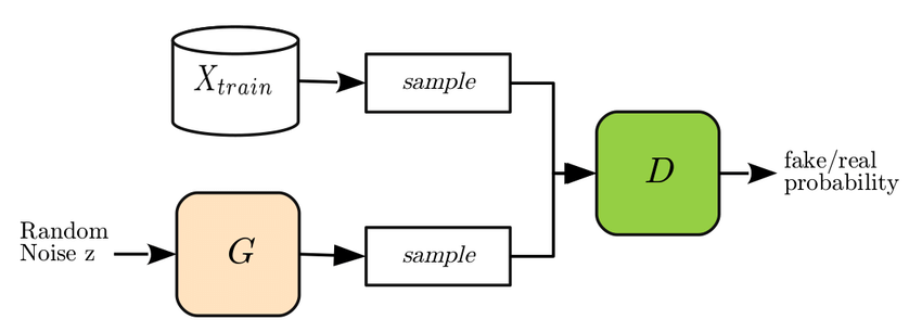
Once the two components are trained, we can either leverage the generator to create synthetic content or the discriminator to identify fake images.
This is cool, but what now?
TL;DR, Yeap, I’ve been there, so, we will build a solution based on two architectures, a generator that creates synthetic images from random noise and a discriminator in charge of identifying real or fake inputs.
For this lab, we will use the MNIST dataset as our ground truth. The MNIST database (Modified National Institute of Standards and Technology database) is a large collection of handwritten digits. It has a training set of 60,000 examples and a test set of 10,000 examples. The images contain grey levels as a result of the anti-aliasing techniques. the images were centered in a 28x28 image by computing the center of mass of the pixels and translating the image to position this point at the center of the 28x28 field. This information is key when setting our architecture parameters.
As for our technology stack, we will use TensorFlow, an open-source library for numerical computation and large-scale machine learning; and Keras, a deep learning API written in Python, running on top of the machine learning platform TensorFlow.
Don’t be scared about the stack, or even if this is the first time you hear about this topic, the goal here is that you can incorporate the main concepts about GANs and their outcome. We will get into Deep Learning and Neural Networks in our next post.
Let’s get our hands dirty
For your reference, I’m using Jupyter Lab on an apple M1. Using the M1 chip, allows me to use the GPU power to run all my projects. If you have an M1/M2 and you want to set up Jupyter to leverage such horsepower, please refer to this tutorial.
As we mentioned before, our core will be Tensorflow and Keras, but we will use some additional libraries that run underneath to help us to manipulate values and plot results.
These are the core set of tools that we will use as part of this project.
from __future__ import print_function, division
from tensorflow.keras.datasets import mnist
from tensorflow.keras.layers import Input, Dense, Reshape, Flatten, Dropout
from tensorflow.keras.layers import BatchNormalization, Activation, ZeroPadding2D
from tensorflow.keras.layers import LeakyReLU
from tensorflow.keras.layers import UpSampling2D, Conv2D
from tensorflow.keras.models import Sequential, Model
from tensorflow.keras.utils import plot_model
from tensorflow.keras.optimizers import Adam
import matplotlib.pyplot as plt
import sys
import os
import numpy as np
import matplotlib.pyplot as plt
import warnings
warnings.filterwarnings('ignore')
%matplotlib inline
%config InlineBackend.figure_format = 'svg'
From Keras, we will import the datasets library which will give us access to the MNIST which is a large database of handwritten digits that is commonly used for training various image processing systems, the layers, optimizers, Models, and some basic tools that will help us to develop the solution. All these libraries are required to build your GAN architecture.
I have included the warnings library to remove undesired messages during execution. This is not required, but it’s nice to avoid those red flags all over the place.
import warnings
warnings.filterwarnings('ignore')
Now, it's time to define some global parameters that will be called by different functions.
As we highlighted previously, the generator is fed by a dense layer that generates random values. That’s why we define a latent_dim of 100.
Next, let’s define our MNIST dataset images’ img_rows, img_cols, and channels. We will use one channel for the images (Gray Scale). For color images using the RGB range, you need to define 3 channels.
Finally, for this lab, we define the optimizer ADAM as a global parameter with a learning rate of 0.0002 and a beta_1 value of 0.5. ,this is a very generic set of values for the optimizer. You can leverage the RMSprop as an alternative and verify the results.
img_rows = 28
img_cols = 28
channels = 1
img_shape = (img_rows, img_cols, channels)
latent_dim = 100
optimizer = Adam(0.0002, 0.5)
#optimizer = optimizers.RMSprop(lr=0.0008, clipvalue=1.0, decay=1e-8)
Now, it's the time of building our generator. We define a function that receives the latent_dim, the height (img_rows), and the width (img_col) of the images as parameters.
As we previously mentioned, Keras is a deep learning API written in Python, running on top of Tensorflow. There are other frameworks such as Pytorch, but something that I really like about Keras is that is straightforward to use for those that are jumping into Deep Learning applied to computer vision for the very first time.
Picture this, you have a set of Legos that you need to put together to build your robot, you have the head, arms, body, legs, etc. Keras is the Legos equivalent of Deep Learning. You add one block on top of another and you build your architecture. (Apologies to my Data Scientist fellows for such an analogy but I think that helps to picture how to build the Keras blocks)
At a high level, the generator is being fed by a dense layer which eventually after going through all the different layers underneath will come up with an image. That image may or may not be a good representation of our ground truth, but as we iterate through the process, our generator will start creating images close to the training set ones.
def build_generator(latent_dim, img_cols, img_rows):
    model = Sequential()
    model.add(Dense(256, input_dim=latent_dim))
    model.add(LeakyReLU(alpha=0.2))
    model.add(Dropout(0.1))
    model.add(BatchNormalization(momentum=0.8))
    model.add(Dense(512))
    model.add(LeakyReLU(alpha=0.2))
    model.add(Dropout(0.1))
    model.add(BatchNormalization(momentum=0.8))
    model.add(Dense(1024))
    model.add(LeakyReLU(alpha=0.2))
    model.add(Dropout(0.1))
    model.add(BatchNormalization(momentum=0.8))
    model.add(Dense(np.prod(img_shape), activation='tanh'))
    model.add(Reshape(img_shape))
    print(model.summary())
    noise = Input(shape=(latent_dim,))
    img = model(noise)
    return Model(noise, img)
As you can see below, this is the result of the first training iteration. We can’t tell whether that’s a number or Super Mario at this stage.
Let’s create our generator object, and get the model summary.
# Build the generator
generator = build_generator(latent_dim, img_cols, img_rows)
plot_model(generator, show_shapes=True, show_layer_names=True)
Model: "sequential_20"
_________________________________________________________________
 Layer (type)                Output Shape              Param #
=================================================================
 dense_71 (Dense)            (None, 256)               25856

 leaky_re_lu_51 (LeakyReLU)  (None, 256)               0

 dropout_3 (Dropout)         (None, 256)               0

 batch_normalization_33 (Bat  (None, 256)              1024
 chNormalization)

 dense_72 (Dense)            (None, 512)               131584

 leaky_re_lu_52 (LeakyReLU)  (None, 512)               0

 dropout_4 (Dropout)         (None, 512)               0

 batch_normalization_34 (Bat  (None, 512)              2048
 chNormalization)

 dense_73 (Dense)            (None, 1024)              525312

 leaky_re_lu_53 (LeakyReLU)  (None, 1024)              0

 dropout_5 (Dropout)         (None, 1024)              0

 batch_normalization_35 (Bat  (None, 1024)             4096
 chNormalization)

 dense_74 (Dense)            (None, 784)               803600

 reshape_11 (Reshape)        (None, 28, 28, 1)         0

=================================================================
Total params: 1,493,520
Trainable params: 1,489,936
Non-trainable params: 3,584
_________________________________________________________________
Now, we will define the discriminator; however, the lab intends to demonstrate how well the generator can create synthetic images from noise. For that purpose, we won’t train the discriminator at this stage, you can train it once the generator is fully trained. The discriminator receives the images' height (img_rows) and width (img_col) as parameters.
def build_discriminator(img_cols, img_rows):
    model = Sequential()
    model.add(Flatten(input_shape=img_shape))
    model.add(Dense(512))
    model.add(LeakyReLU(alpha=0.2))
    model.add(Dense(256))
    model.add(LeakyReLU(alpha=0.2))
    model.add(Dense(1, activation='sigmoid'))
    print(model.summary())
    img = Input(shape=img_shape)
    validity = model(img)
    return Model(img, validity)
Similar to what we did with our generator, we will build the object. The main difference is that we need to set the compilation parameters which includes the loss function and the optimizer defined above (ADAM), which will be used during the discriminator training process.
# Build and compile the discriminator
discriminator = build_discriminator(img_cols, img_rows)
discriminator.compile(loss='binary_crossentropy',optimizer=optimizer,metrics=['accuracy'])
plot_model(discriminator, show_shapes=True, show_layer_names=True)
Now, let’s set up some additional parameters. As we mentioned, we want to train the generator first, so we must set the discriminator.trainable = False
The whole magic behind the GAN is that the solution takes random noise from a low-dimensionality array and generates images from it.
On the other hand, the discriminator takes the images created by the generator and determines whether those are real or fake.
The entire model is combined within one single variable combined = Model(z, validity) which includes the latent space and the validity to train both components.
# For the combined model we will only train the generator
discriminator.trainable = False

# The generator takes noise as input and generates imgs
z = Input(shape=(latent_dim,))
img = generator(z)

# The discriminator takes generated images as input and determines validity
validity = discriminator(img)

# The combined model  (stacked generator and discriminator)
# Trains the generator to fool the discriminator
combined = Model(z, validity)
combined.compile(loss='binary_crossentropy', optimizer=optimizer)
Dude, I’m tired already
Yeap, I get it but bear with me for a few minutes. We are almost there.
Now we need to define another function to save the images and the main code which will call out the training process.
This function will save the images in the images directory. If the directory does not exist, it will create one for you.
def sample_images(epoch):
    r, c = 5, 5
    noise = np.random.normal(0, 1, (r * c, latent_dim))
    gen_imgs = generator.predict(noise)

    # Rescale images 0 - 1
    gen_imgs = 0.5 * gen_imgs + 0.5
    fig, axs = plt.subplots(r, c)
    cnt = 0
    for i in range(r):
        for j in range(c):
            axs[i,j].imshow(gen_imgs[cnt, :,:,0], cmap='gray')
            axs[i,j].axis('off')
            cnt += 1

    # If images directory does not exist, create one
    if not os.path.isdir("images"):
        os.makedirs("images")

    fig.savefig("images/%d.png" % epoch)
    plt.close()
We talk a lot about MNIST, but we haven’t loaded the data yet. It’s time to bring our ground truth dataset into the game.
# Load the dataset
(X_train, _), (_, _) = mnist.load_data()

# Rescale -1 to 1
# Expand the X_train in one additional dimension
X_train = X_train / 127.5 - 1.
X_train = np.expand_dims(X_train, axis=3)
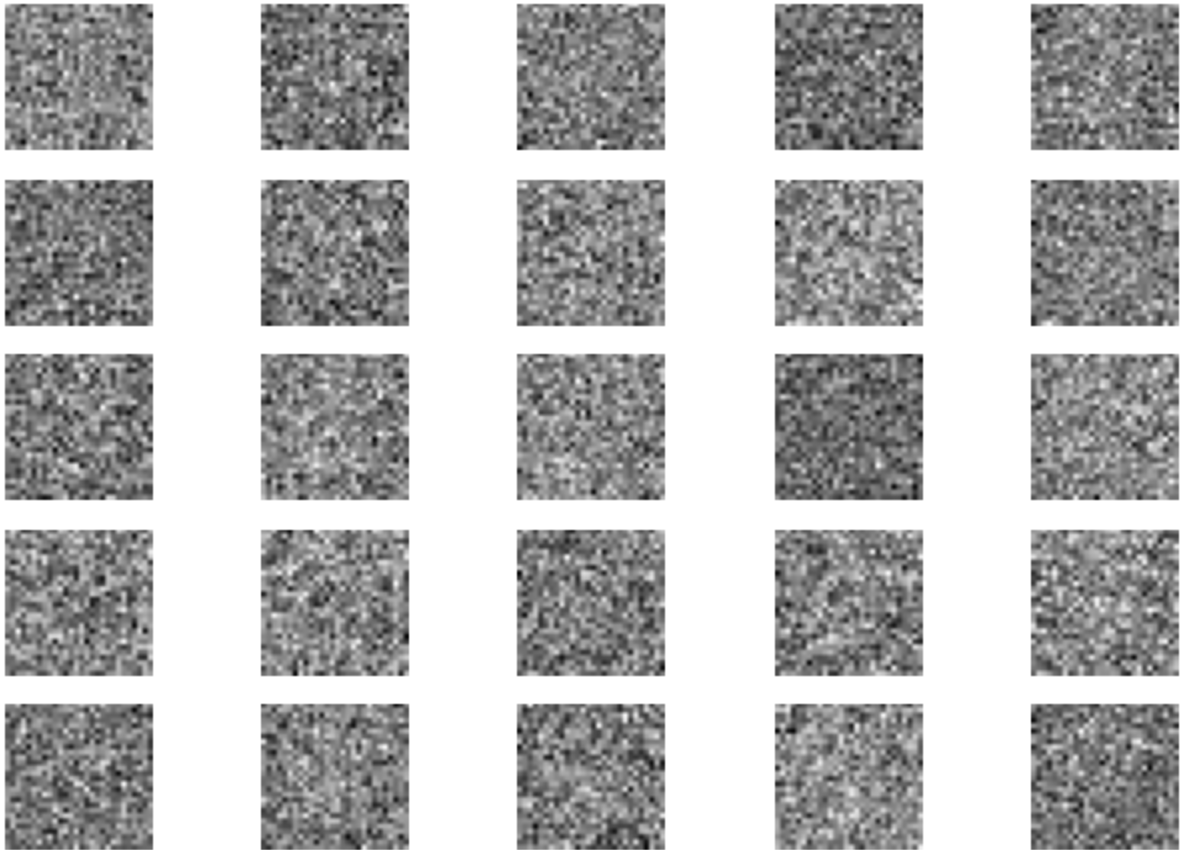
Let’s plot the first 9 images from our dataset. We will see some of the handwritten inputs loaded into the MNIST data set.
# Training set visualization
# We plot first 9 images of training dataset
plt.figure(figsize =(5, 5))
for i in range(9):
    plt.subplot(330 + 1 + i)
    plt.imshow(X_train[i], cmap=plt.get_cmap('gray'))
plt.show()
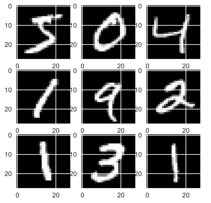
MNIST dataset
What have we got so far?
Generator
Discriminator
Function to save synthetic images
Load the MNIST dataset
Normalize the Data
Plot the first 9 numbers from the dataset
Now is the time to bring the mother of all the functions, which will be in charge of running the show for us.
I’ll try to summarize the overall process for you. First I want to recognize our colleague Erik Linder-Norén for his contribution to developing Machine Learning content. I leverage some ideas from his work.
The train function receives the training dataset, the number of epochs, the batch_size (by default 128), and the sample_interval (by default 50).
The epochs are the number of cycles that the training process will last. The iterations and the outcome is hard to define, so you will find different recommendations depending on the use case, it’s not the same running 3000 epochs for this problem than 3000 epochs to generate RGB images.
The batch_size tells you the size of data that will be loaded on each epoch.
The sample_interval is a variable used as a reference to save images depending on the epoch we are located at.
The entire goal of the GAN is to not only generate synthetic images but to let the discriminator identify whether those images are real or fake. That’s the adversarial game. For that purpose, we identify valid images with the label of 1 and fake images with the label of 0.
The two main sections are the discriminator and generator training blocks.
During the discriminator training process, the discriminator receives images from the MNIST dataset flagged 1 and synthetic versions created by our generator flagged as 1 well, but the discriminator has to identify whether the latter is fake or not. If our police-bot can identify the fake image, it will let the generator know so the next time the generator creates better instances.
The second part is the generator training process. Here, the generator is fed with the noise produced by noise = np.random.normal(0, 1, (batch_size, latent_dim)), and that data is used by the generator to eventually come up with an image that may be similar to our ground truth.
for both, we store and show the loss functions which are showcased during the training process.
  def train(X_train,
          epochs,
          batch_size=128,
          sample_interval=50):

        # Adversarial ground truths
        valid = np.ones((batch_size, 1))
        fake = np.zeros((batch_size, 1))

        for epoch in range(epochs):

            # ----------------------------------------------------
            #  Train Discriminator
            # discriminator.trainable = False must be set to True
            # ----------------------------------------------------

            # Select a random batch of images
            idx = np.random.randint(0, X_train.shape[0], batch_size)
            imgs = X_train[idx]

            noise = np.random.normal(0, 1, (batch_size, latent_dim))

            # Generate a batch of new images
            gen_imgs = generator.predict(noise)

            # Train the discriminator
            d_loss_real = discriminator.train_on_batch(imgs, valid)
            d_loss_fake = discriminator.train_on_batch(gen_imgs, fake)
            d_loss = 0.5 * np.add(d_loss_real, d_loss_fake)

            # ---------------------
            #  Train Generator
            # ---------------------

            noise = np.random.normal(0, 1, (batch_size, latent_dim))

            # Train the generator (to have the discriminator label samples as valid)
            g_loss = combined.train_on_batch(noise, valid)

            # Plot the progress
            print ("%d [D loss: %f, acc.: %.2f%%] [G loss: %f]" % (epoch, d_loss[0], 100*d_loss[1], g_loss))

            # If at save interval => save generated image samples
            if epoch % sample_interval == 0:
                sample_images(epoch)
And, now is showtime! Let’s call the train function with the following parameters. You can adapt these parameters according to your needs.
X_train(our ground truth MNIST)epochs=5000batch_size=32sample_interval=200
train(X_train, epochs=5000, batch_size=32, sample_interval=200)
Once you run this final code block, you will start seeing the training process outcome.
GAN training process
Epoch 1 result
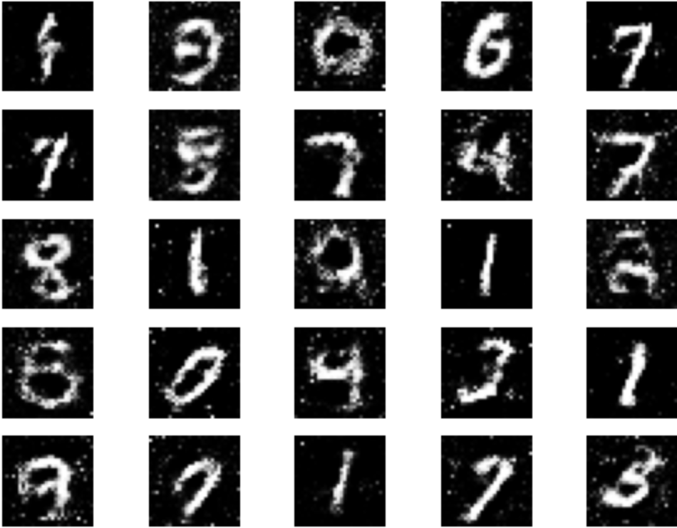
After some epochs, you should start seeing some interesting results. As you can see at epoch 1000, while there are a few entries that make no sense, we can identify some instances that seem numbers, similar to our ground truth, like 6, 9, 1, or even 8 What about if we go further in the process?

Epoch 1000
Epoch 3000
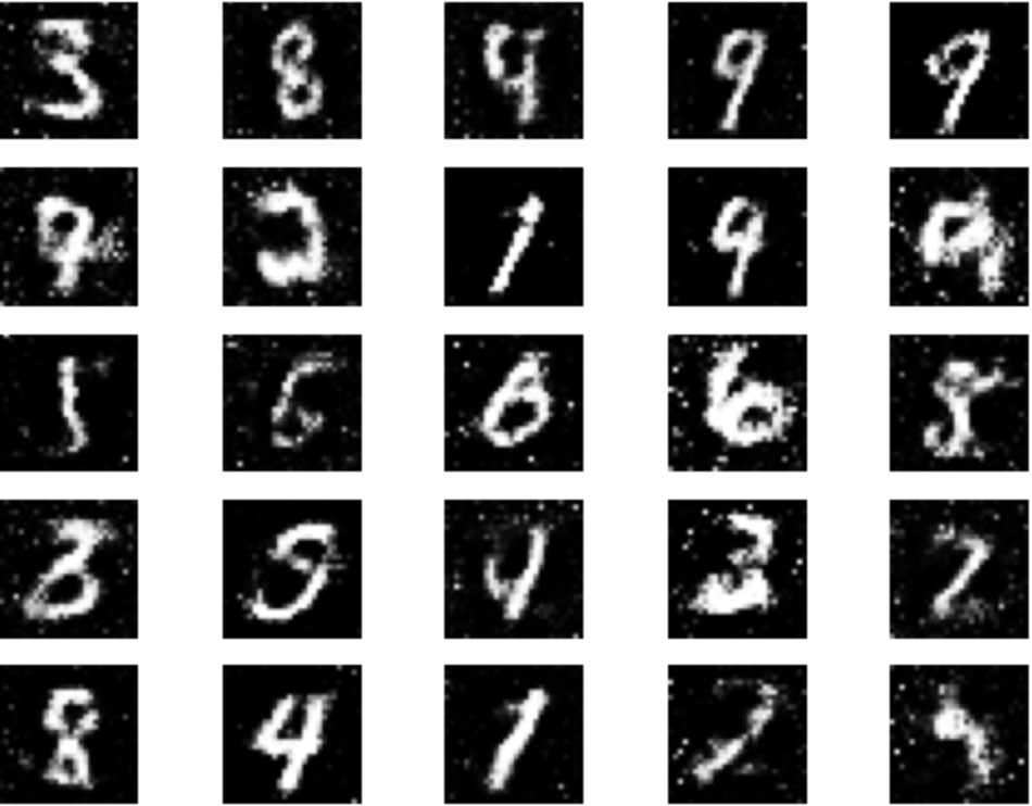
Epoch 5000
As we move forward, even though we still see a few entries that seem scribbled, there are other entries very well-defined compared to the first training epochs, such as 4, 8, 6, 9 and 1
Fascinating, right? With a few lines of code, we actually create content from noise. We are on the verge of a computing transformation as we know it as GANs, Autoencoders, and Transformers keep evolving, and we expect that solutions like ChatGPT or DALL-E2 become a complement to our daily lives. But regardless of the technology, everything starts somewhere, and here you will find the first step that will help you to move in that direction and seek further information. And remember, don’t stress out, just enjoy the ride.
Hope you have found this post informative. Feel free to share it, we want to reach as many people as we can because knowledge must be shared, right?
If you reach this point, Thank you!
<AL34N!X>